
Reducing LLM Inference Costs: Batching and Parallelism #
Running LLMs in production is expensive and its not a model problem it’s a systems problem.
On AWS, GPU instances vary widely in cost. High-end inference nodes like an EC2 p4d.24xlarge with 8× A100 GPUs can run ~$25–35/hr on-demand, while a single-GPU instance such as g5.xlarge runs ~$1/hr on-demand about $700+ per month if left running 24/7.
When GPUs run continuously, small inefficiencies compound quickly. In poorly optimized systems, this means the cost per token drastically increases.
Hence the focus must shift from model quality to GPU utilization, memory bandwidth efficiency and Scheduling and request orchestration.
Some of the core techniques that reduce inference costs are - Batching, Parallelism, Memory bandwidth optimization and eleminating idle GPU time.
This post covers the following techniques that reduce inference costs:
- Batching: Processing multiple requests together
- Parallelism: Distributing work across GPU resources
Why GPUs Are Both Fast and Wasteful #
GPUs are designed for massive parallel throughput, not low-latency single-request execution.
Take the NVIDIA A100 (commonly used in AWS p4d instances):
- 6,912 CUDA cores for parallel computation
- 80GB HBM2e memory with 2TB/s bandwidth
- 312 TFLOPS of FP16 compute
The problem - most inference workloads use only a fraction of that capacity.
Single Request Inference:
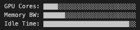
When you process a single request, most GPU cores sit idle while waiting for:
- Memory transfers - loading model weights
- Sequential operations - attention computations
- I/O operations - tokenization, network
The Economics of LLM Inference #
Before diving into techniques, let’s understand the cost structure.
LLM inference cost is not determined by model size alone. It is determined by how efficiently you convert GPU time into tokens.
On AWS, you are billed primarily for GPU instance uptime and not for tokens generated. That means the real optimization target is tokens per GPU-dollar.
Cost_per_token ∝ 1 / (tokens_per_second)
Example:
Before optimization:
- g5.xlarge = $1/hr
- Lets assume - model produces
100 tokens/sec
In one hour : 100 * 3600 = 360,000 tokens
Cost per token = $1/360,000 = $0.00000278 per token
After optimization:
Lets assume - model produces 400 tokens/sec
In one hour : 400 * 3600 = 1,440,000 tokens
Cost per token = $1 / 1,440,000 ≈ $0.00000069 per token
If you notice from the above math - We reduced cost per token by 4X, without changing model size and without changing hardware. Only by increasing throughput.
If throughput doubles, cost per token is halved — assuming the instance cost remains constant.
| Cost Factor | Description | Impact |
|---|---|---|
| GPU Hours | Time your EC2 GPU instance is running | Direct billing cost |
| Token Processing | Tokens generated per second | Determines cost per token |
| Memory Bandwidth | How fast weights and KV cache move through High Bandwidth Memory | Bottleneck for large models |
| Idle GPU Time | Cores waiting for data | Wasted compute capacity |
In production, the goal is not “fast inference.”, it’s the following:
- Maximize tokens per GPU second
- Minimize idle time
- Avoid memory-bound stalls
- Meet latency constraints without sacrificing utilization
Batching: The Foundation of Efficient Inference #
Batching increases arithmetic intensity and GPU saturation which directly increases tokens/sec and lowers cost per token.
What Is Batching? #
Batching means processing multiple requests simultaneously instead of one at a time. This amortizes the fixed costs (loading weights, kernel launches) across multiple outputs.
Without Batching (Sequential):
Request 1 → [Load Weights] → [Compute] → [Output]
Request 2 → [Load Weights] → [Compute] → [Output]
Request 3 → [Load Weights] → [Compute] → [Output]
Total: 3x weight loading, 3x kernel overhead
With Batching:
Requests 1,2,3 → [Load Weights Once] → [Parallel Compute] → [Outputs]
Total: 1x weight loading, 1x kernel overhead
Static vs Dynamic Batching #
Static Batching: #
Static batching groups requests into a fixed-size batch - The system waits until N requests arrive. Once the batch is full, it pads all sequences to the same length, runs a forward pass, and then returns the outputs.
Flow:
- Wait until N requests arrive
- Pad sequences to equal length
- Run forward pass
- Return outputs
This works well when request sizes are similar and traffic is steady. It’s simple to implement and easy to reason about. Many early inference systems use this approach.

But static batching has two structural problems.
- First, it introduces queueing latency. If your batch size is 32, and only 20 requests have arrived, the GPU waits. You are trading latency for throughput.
- Second, and more importantly - it suffers from the padding problem.
Padding Problem
LLMs operate on tensors with uniform dimensions. That means every sequence in a batch must have the same length. If requests have different token counts, the shorter ones are padded to match the longest.
Example:
Req1: 120 tokens
Req2: 60 tokens
Req3: 20 tokens
In Static batch tensor size - Thhe Batch size = 3 and the Sequence length = 120, which means Req2 wastes 60 token positions and Req3 wastes 100 token positions.
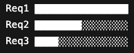
The GPU performs computation on positions that carry no useful information. This is not just wasting compute, but also consuming memory bandwidth and occupying Tensor Cores with zeros. As variation in request length increases, static batching becomes increasingly inefficient.
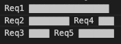
Dynamic/Continuous Batching: #
Instead of batching entire requests together and waiting for them to finish, the scheduler operates at the token level.
When a request finishes generating its final token, its slot in the batch becomes immediately available. A new request can be inserted into that position in the next decoding step.
There is no need to wait for N full requests to accumulate. There are no large padding gaps for sequences that ended early. The GPU remains saturated because there are always active sequences occupying its compute slots.
This approach is used in modern inference engines like vLLM.
Pros
- Lower queueing latency
- Higher sustained GPU utilization
- Reduced padding waste
- Better throughput under uneven traffic
Cons
- Fine-grained scheduling
- Careful KV cache management
- Token-level execution control
- More complex memory bookkeeping
Static batching is easy and works well when traffic is uniform and predictable.
Continuous batching is adaptive. It handles variable request lengths, bursty traffic, and real-world workload patterns without letting the GPU sit idle.
Parallelism Strategies for LLM Inference #
Batching makes a single GPU more efficient. But what to do when one GPU is not enough - for example - if the model is too large to fit into one GPU’s memory, or the traffic volume is too high for a single device to handle - that’s where we use parallelism.
Example - From a single g5.xlarge to multi-GPU instances like p4d.24xlarge, or scale horizontally across multiple nodes
Data Parallelism #
The simplest strategy is to replicate the full model on multiple GPUs and distribute requests across them. Each GPU has its own copy of the weights in High Bandwidth Memory. Each one processes batches independently. If one GPU can handle 300 tokens per second, two GPUs can handle roughly 600. The scaling is close to linear, assuming traffic is steady enough to keep all GPUs busy.
This works well when:
- The model fits comfortably into a single GPU’s memory
- Traffic volume is high and predictable
- You want simple autoscaling
The tradeoff
Every GPU needs enough memory to hold the entire model. If you deploy an 80GB model across 8 GPUs, you are allocating 640GB of aggregate GPU memory, even though each copy is identical and if traffic drops there will be expensive GPUs sitting idle.
Well the advantage of Data Parallelism approach is - Its Simple, linear throughput scaling but the disadvantage is - Each GPU needs full model memory, high memory cost.
Tensor Parallelism - Splitting the Model Itself #
When a model no longer fits into a single GPU, replication stops working. You cannot load what does not fit.
Tensor parallelism solves this by splitting large weight matrices across multiple GPUs.
Instead of one GPU computing the full matrix multiplication, each GPU computes a slice of it. The results are then combined through high-speed interconnects like NVLink.
This means - One GPU holds part of the weights. Another GPU holds the rest. Together, they compute what neither could alone. This allows you to run much larger models, but it introduces a new cost that is communication .
Every forward pass now requires GPUs to synchronize and exchange partial results. If the interconnect is slow, performance suffers. On tightly coupled instances like AWS p4d with NVLink, this works well. But across separate nodes the network overhead becomes significant.
Well the advantage of Tensor parallelism is it - enables larger models, but the disadvantage is it increases system complexity and communication sensitivity.
Pipeline Parallelism - Layer-by-Layer Distribution #
This strategy is to divide the model by layers instead of tensors. GPU 0 runs the first set of layers. GPU 1 runs the next set. GPU 2 runs the final layers. The output of one becomes the input to the next. This allows extremely large models to run by spreading memory requirements across devices.
However, it introduces pipeline bubbles — moments when some GPUs are waiting while others are working. Latency also increases because each request must travel through the entire chain.
This strategy is typically used when models are so large that other options are insufficient.
The Hidden Tradeoff of Paralelism - Compute vs Communication
Parallelism always introduces coordination overhead. If communication cost grows faster than compute then scaling becomes a over head with increase in cost, by simply adding GPU’s.
Parallelism only improves economics when - GPUs remain highly utilized, Communication overhead is minimized and Throughput scales proportionally with hardware.
| Stategy | Usecase |
|---|---|
| Data Parallelism | horizontal scaling |
| Tensor Parallelism | when model size outgrows |
| Pipeline Parallelism | The need of the hour for very large models |
Choosing the Right Strategy #
| Scenario | Recommended Parallelism |
|---|---|
| Model fits on 1 GPU, need throughput | Data Parallelism |
| Model too large for 1 GPU, low latency needed | Tensor Parallelism |
| Very deep model, multiple GPUs available | Pipeline Parallelism |
Popular Inference Frameworks #
| Framework | Key Features | Best For |
|---|---|---|
| vLLM | PagedAttention, continuous batching | High-throughput serving |
| TensorRT-LLM | NVIDIA optimizations, INT4/INT8 | NVIDIA GPU production |
| Text Generation Inference | Rust performance, easy deployment | Hugging Face models |
| llama.cpp | CPU/Metal support, quantization | Local/edge deployment |
Further Reading #
- Continuous Batching - Anyscale blog
- LLM Inference Performance Engineering - Comprehensive overview
- NVIDIA TensorRT-LLM - Production-grade inference